Work / Putting broken 3D objects back together
Putting broken 3D objects back together
Honours thesis: Multi-Hypothesis Consensus Refinement for SE(3) Flow Matching in 3D Fragment Reassembly
A training-free method that makes a 3D reassembly model more reliable by letting it vote on where each piece goes.
| Type | Honours thesis, University of Sydney |
|---|---|
| Supervisor | A/Prof. Weidong Cai |
| Timeline | Jun 2025 – May 2026 |
| Result | Completed, First Class Honours (mark 88) |
| Stack | Python, PyTorch, PyTorch3D, Point Transformer V3, Open3D |
| Code | Lab repository, not public |
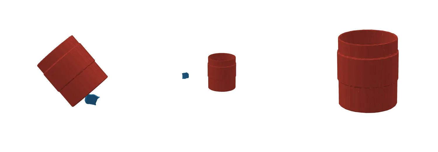
Illustration: a vase made of points is broken into seven pieces. One piece stays fixed, and the other six move back into place one at a time, each turning and sliding until it fits.
The problem
You are given the scattered pieces of a broken object, each turned and moved by an unknown amount. The job is to work out how to rotate and move every piece so they fit back together. It matters for digital restoration of pottery and sculpture, forensic reconstruction and the analysis of mechanical failures.
It is harder than it looks:
- Neighbouring pieces only touch along their fracture surfaces. Their outer surfaces never overlap, so ordinary point-cloud matching has nothing to hold on to.
- Every piece has to be placed jointly and consistently with the others.
- Symmetric objects such as bottles, bowls and vases allow many equally plausible answers.
- More pieces make it much harder.
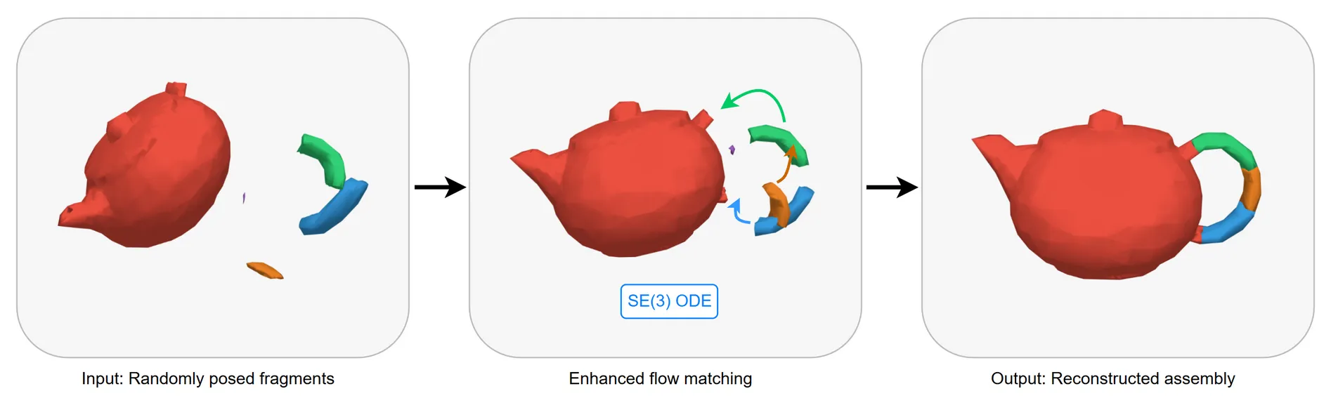
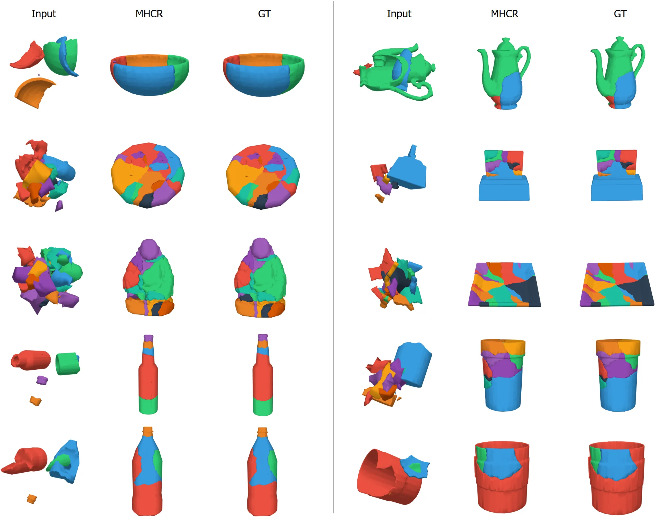
I worked on the Breaking Bad benchmark (the Everyday subset, 20 object categories), which comes in two splits: volume-constrained, with up to about 20 similar-sized pieces, and the harder vanilla, with 2 to 50 pieces of very uneven size.
The idea: let the model vote
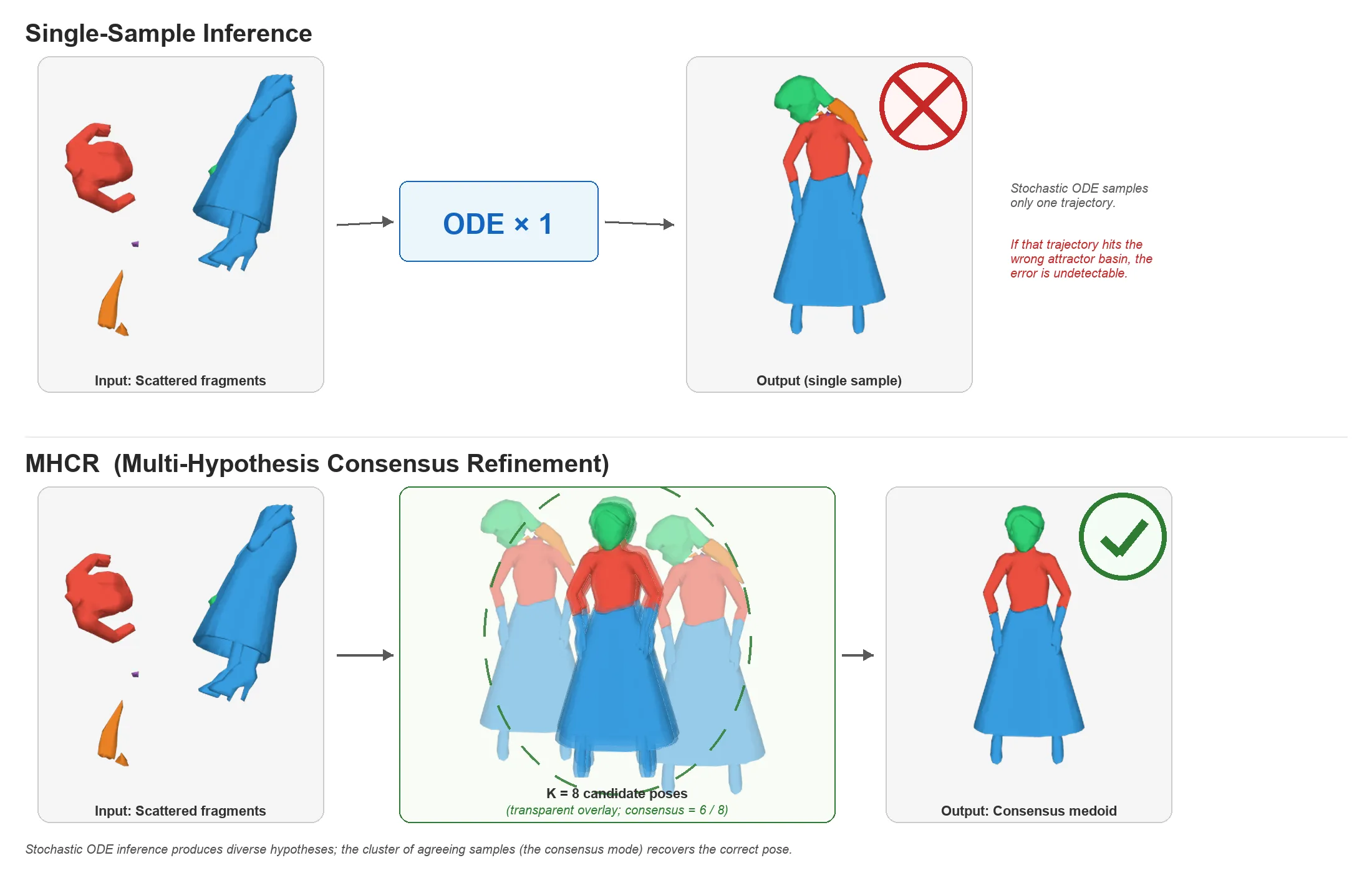
The starting point was GARF (ICCV 2025), a flow-matching model and the strongest reassembly method with public code when I began. It solves the puzzle once, starting from random noise. A different random start can land on a different answer, and a single run can be confidently wrong with no warning.
My method, MHCR (Multi-Hypothesis Consensus Refinement), turns that randomness into a confidence signal. It needs no retraining:
- Read the pieces’ shapes once.
- Solve the puzzle 8 times from different random starts.
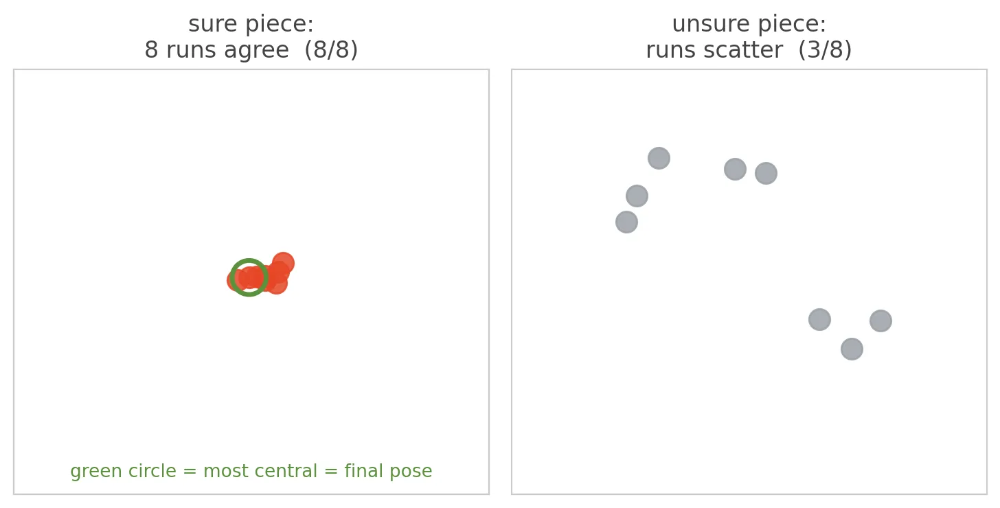
- For each piece, check whether the answers agree. If most of them agree, trust that answer.
- Lock the trusted pieces as a scaffold and solve again for only the doubtful ones around them.
- Repeat until no more pieces get locked.
Once most of the pieces are in place, the last few are easy.
1Read the pieces
- Point Transformer V3 encoder
- Runs once per object
2Solve 8 times
- SE(3) flow matching
- Different random starts
3Check agreement
- Cluster each piece’s rotations
- Agreement becomes confidence
4Lock a scaffold
- Keep the confident pieces fixed
- Re-solve the doubtful ones
5Output
- One pose per piece
- No retraining needed
Steps 2 to 4 repeat until no new piece gets locked, for up to 6 rounds.
I also added three small extensions to the model’s denoiser: per-point attention to the encoder’s features, a token marking fracture surfaces, and an injection of the encoder’s bottleneck features. After fine-tuning, they added 0.88 points of part accuracy on the full volume-constrained validation set, averaged over 5 seeds.
Results
Part accuracy is the share of pieces placed within a small error of the true pose, averaged per object. Every comparison below is against GARF re-run under identical settings.
Gain in part accuracy over GARF, in points (easier at the top, harder at the bottom)
- Volume-constrained, up to 20 pieces+1.592.1% → 93.6% part accuracy, single run
- Vanilla, up to 20 pieces+2.989.6% → 92.5% part accuracy, single run
- 3-category subset, 5 seeds+3.891.0% → 94.8% part accuracy, mean of 5 seeds
- Vanilla, 21–33 pieces (hardest)+14.160.6% → 74.7% part accuracy, single run
| Measure | Value | Context |
|---|---|---|
| Vanilla, 21–33 pieces (hardest) | 60.6% → 74.7% | +14.1 points, single run |
| Vanilla, up to 20 pieces | 89.6% → 92.5% | +2.9 points, single run |
| 3-category subset (vanilla) | 91.0% → 94.8% | +3.8 points, mean of 5 seeds |
| Volume-constrained, up to 20 pieces | 92.1% → 93.6% | +1.5 points, single run |
| Denoiser extensions alone | +0.88 points | Full volume-constrained validation set, 5 seeds |
Baseline: GARF (ICCV 2025), the strongest open-source method when the work began, re-run with the same data, filters and metric.
What I learned along the way
- A pivot after months of dead ends. The project started as learned point-cloud compression, then a fragment-token autoencoder. Its surfaces kept coming out blocky or half-formed. In late March 2026 I moved to the standard reassembly benchmark so the work could be compared with published methods.
- Making rotations learnable. My first diffusion and flow models stalled at the “do nothing” baseline because rotations were being interpolated in a way that isn’t valid for rotations. Switching to geodesic flow matching on rotations fixed the formulation. The same debugging found two more bugs: mixed precision was killing the rotation gradients, and a weight-decay setting far too high was crushing the rotation head.
- Why fix-up stages failed, and where the idea came from. Supervised refinement stages learned the average of the valid answers for symmetric pieces, or learned to change nothing. The insight was that different random starts land on different answers, and the right one is usually among them.
- Context beats brute force. At similar compute, 8 runs with scaffold rounds placed 85.7% of pieces within tight tolerances, against 76.5% for 32 independent runs. What helps is context, not more samples.
- Catching my own false positive. One experiment showed a suspiciously large gain while its control scored far below the published baseline. The cause was a locally regenerated data file whose training and validation objects overlapped completely. I switched every script to the official data, deleted the affected checkpoints and wrote the pitfall down.
- An honest negative study. I tested 22 inference-time refinement strategies: 4 helped, 9 made no difference and 9 hurt. Most of the remaining errors come from near-symmetric pieces such as bottles and vases.
Preparing the data
Before any model could train, every object needed the same format. I wrote a batch pipeline that turned 542 meshes from 20 categories into 2,048-point clouds with surface normals. It cleans each mesh, “scans” it from 36 virtual camera views on the GPU so only the visible outer surface is kept, thins the result to exactly 2,048 well-spread points, and saves each object under a predictable name. A broken input is reported and skipped instead of stopping the batch.
1Load the mesh
- Remove duplicate and degenerate faces
- Skip and report broken inputs
2Virtual scan
- 36 camera views, rendered on the GPU (PyTorch3D)
- Keep only the visible outer surface
3Resample
- Farthest-point sampling to 2,048 points
- Estimate consistent normals
4Save
- One file per object
- Consistent names, progress log
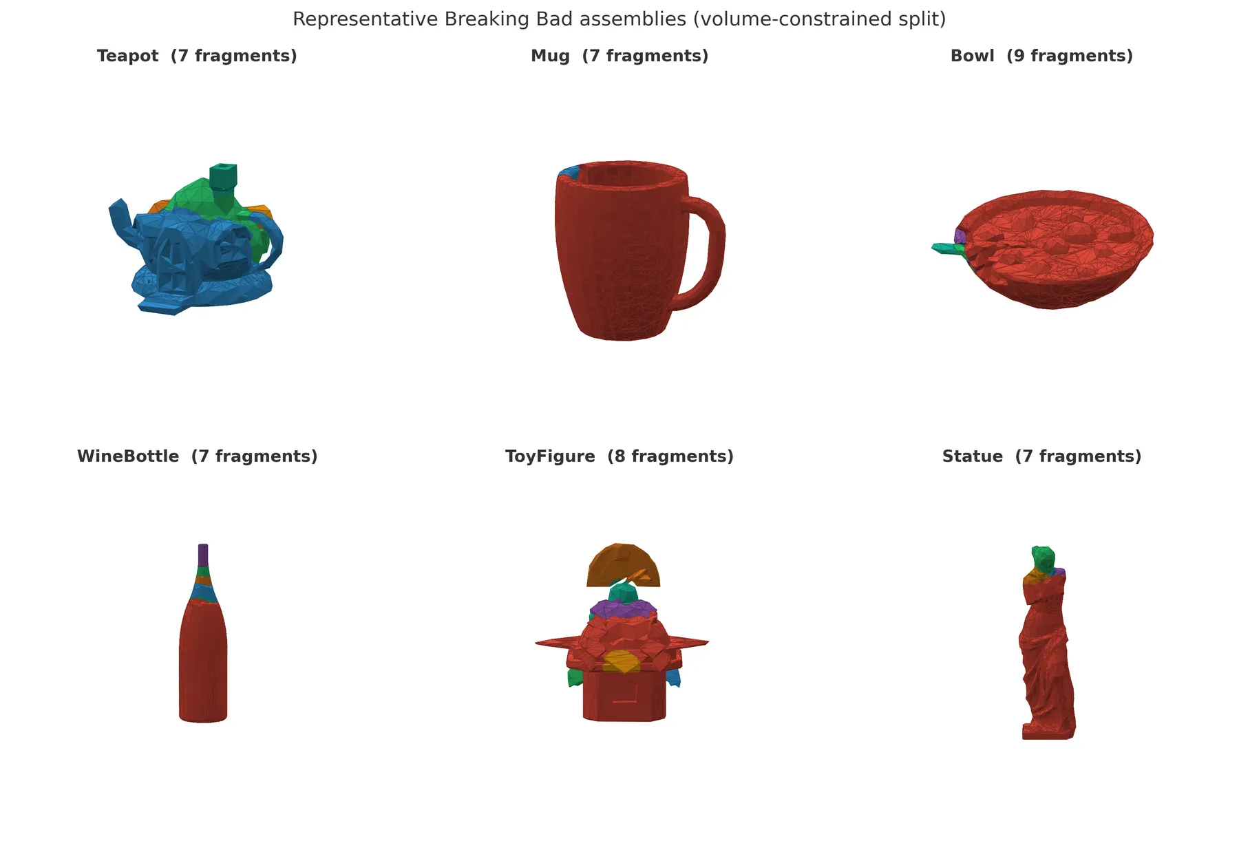
Gallery
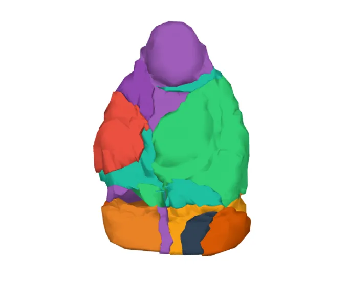
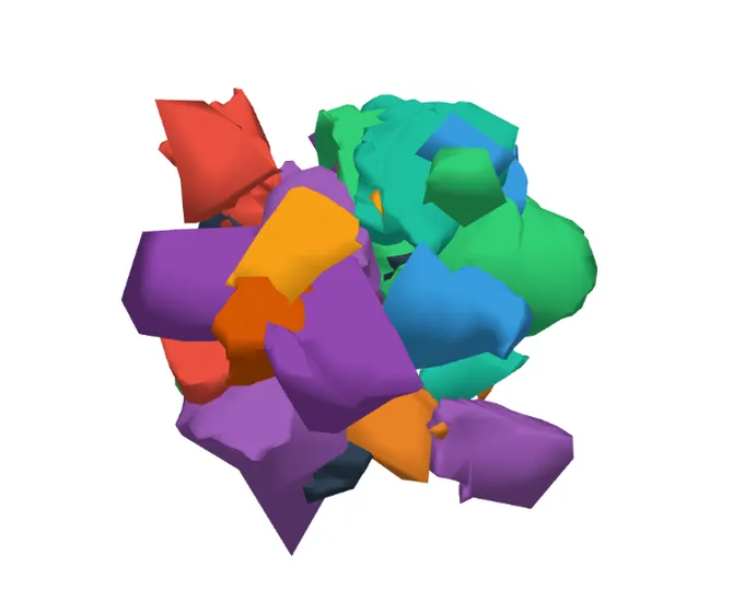
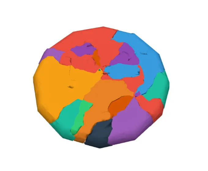
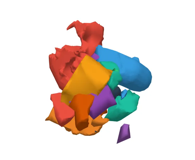
Supervised by A/Prof. Weidong (Tom) Cai, with day-to-day mentoring from Wei Guo, whose discussions helped shape the consensus idea. Dataset: Breaking Bad (Sellán et al., NeurIPS 2022). Baseline: GARF (ICCV 2025). Thesis submitted to the School of Computer Science, The University of Sydney, May 2026.